Climate Vulnerability Modeling in Malawi

Replication of Malcomb Vulnerability Modeling in Sub-Saharan Africa

Original study by Malcomb, D. W., E. A. Weaver, and A. R. Krakowka. 2014. Vulnerability modeling for sub-Saharan Africa: An operationalized approach in Malawi. Applied Geography 48:17–30. DOI:10.1016/j.apgeog.2014.01.004

Replication Authors: Nick Nonnenmacher, Joseph Holler, Kufre Udoh, Open Source GIScience students of fall 2019 and Spring 2021

Replication Materials Available at: nicknonnen/RP-Malcomb

Created: 14 April 2021 Revised: 28 April 2021

Acknowledgements

Thank you Kufre Udoh and Professor Joe Holler of Middlebury College for providing a robust framework for the R script used in this study, and for organizing data and a collaborative work environment for completing this reproduction. I would also like to thank my lab group, including Maja Cannavo, Emma Clinton, Drew An-Pham, Jacob Freedman, and Alitzel Villaneuva, for their assistance in designing our R script workflow, creating final figures and tables, overcoming coding challenges, and collaboratively compiling data transformation, source, and variable descriptions.

Abstract

The original study is a multi-criteria analysis of vulnerability to Climate Change in Malawi, and is one of the earliest sub-national geographic models of climate change vulnerability for an African country. The study aims to be replicable, and had 40 citations in Google Scholar as of April 8, 2021.

Original Study Information

The study region is the country of Malawi. The spatial support of input data includes DHS survey points, Traditional Authority boundaries, and raster grids of flood risk (0.833 degree resolution) and drought exposure (0.416 degree resolution).

The original study was published without data or code, but has detailed narrative description of the methodology. The methods used are feasible for undergraduate students to implement following completion of one introductory GIS course. The study states that its data is available for replication in 23 African countries.

Data Description and Variables

This section was produced collaboratively with labmates Maja Cannavo, Emma Clinton, Drew An-Pham, Jacob Freedman, and Alitzel Villaneuva.

Access and Assets Data

Demographic and Health Survey data are a product of the United States Agency for International Development (USAID). Variables contained in this dataset are used to represent adaptive capacity (access + assets) in the Malcomb et al.’s (2014) study. These data come from survey questionnaires with large sample sizes.

The DHS data used in our study were collected in 2010. In Malawi, the provenance of the DHS data dates back as far as 1992, but has not been collected consistently every year. Each point in the household dataset represents a cluster of households with each cluster corresponding to some form of census enumeration units, such as villages in rural areas or city blocks in urban areas DHS GPS Manual. This means that each household in each cluster has the same GPS data, and that while the data collected carries a high degree of precision, it may not be accurately spatially representing target populations. This data is collected by trained USAID staff using GPS receivers.

Missing data is a common occurrence in this dataset as a result of negligence or incorrect naming. However, according to the DHS GPS Manual, these issues are easily rectified and typically sites for which data does not exist are recollected. Sometimes, however, missing information is coded in as such or assigned a proxy location.

The DHS website acknowledges the high potential for inconsistent or incomplete data in such broad and expansive survey sets. Missing survey data (responses) are never estimated or made up; they are instead coded as a special response indicating the absence of data. As well, there are clear policies in place to ensure the data’s accuracy. More information about data validity can be found on the DHS’s Data Quality and Use site. In this analysis, we use the variables listed in Table 1 to determine the average adaptive capacity of each TA area. Data transformations are outlined below.

Metadata source: Burgert, C. R., Zachary, B., Colston, J. The DHS Program—Data. (2010). The DHS Program–USAID. Retrieved April 19, 2021, from https://dhsprogram.com/Data/ and DHS_GPS_Manual_English_A4_24May2013_DHSM9.pdf file in metadata

Table 1: DHS Variables used in Analysis

Variable Code	Definition
HHID	“Case Identification”
HV001	“Cluster number”
HV002	Household number
HV246A	“Cattle own”
HV246D	“Goats own”
HV246E	“Sheep own”
HV246G	“Pigs own”
HV248	“Number of sick people 18-59”
HV245	“Hectares for agricultural land”
HV271	“Wealth index factor score (5 decimals)”
HV251	“Number of orphans and vulnerable children”
HV207	“Has Radio”
HV243A	“Has a Mobile Telephone”
HV219	Sex of Head of Household”
HV226	“Type of Cooking Fuel”
HV206	“Has electricty”
HV204	“Time to get to Water Source”

Variable Transformations

1. Eliminate households with null and/or missing values
2. Join TA and LHZ ID data to the DHS clusters
3. Eliminate NA values for livestock
4. Sum counts of all different kinds of livestock into a single variable
5. Apply weights to normalized indicator variables to get scores for each category (assets, access)
6. find the stats of the capacity of each TA (min, max, mean, sd)
7. Join ta_capacity to TA based on ta_id
8. Prepare breaks for mapping
9. Class intervals based on capacity_2010 field
10. Take the values and round them to 2 decimal places
11. Put data in 4 classes based on break values

Livelihood Zones Data

The livelihood zone (LHZ) data is created by aggregating general regions where similar crops are grown and similar ecological patterns exist. This data exists originally at the household level and was aggregated into Livelihood Zones. To construct the aggregation used for “Livelihood Sensitivity” in this analysis, we use these household points from the FEWSNet data that had previously been aggregated into livelihood zones.

The four Livelihood Sensitivity categories are 1) Percent of food from own farm (6%); 2) Percent of income from wage labor (6%); 3) Percent of income from cash crops (4%); and 4) Disaster coping strategy (4%). In the original R script, household data from the DHS survey was used as a proxy for the specific data points in the livelihood sensitivity analysis (transformation: Join with DHS clusters to apply LHZ FNID variables).

The LHZ data variables are outlined in Table 2. The four categories used to determine livelihood sensitivity were ranked from 1-5 based on percent rank values and then weighted using values taken from Malcomb et al. (2014).

Metadata source: Malawi Baseline Livelihood Profiles, Version 1* (September 2005). Made by Malawi National Vulnerability Assessment Committee in collaboration with the SADC FANR Vulnerability Assessment Committee (mw_baseline_rural_en_2005.pdf file in metadata)

Table 2: Constructing Livelihood Sensitivity Categories

Livelihood Sensitivity Category (LSC)	Percent Contributing	How LSC was constructed
Percent of food from own farm	6%	Sources of food: crops + livestock
Percent of income from wage labor	6%	Sources of cash: labour etc. / total * 100
Percent of income from cash crops	4%	sources of cash (Crops): (tobacco + sugar + tea + coffee) + / total sources of cash * 100
Disaster coping strategy	4%	Self-employment & small business and trade: (firewood + sale of wild food + grass + mats + charcoal) / total sources of cash * 100

Variable Transformations

1. Join with DHS clusters to apply LHZ FNID variables
2. Clip TA boundaries to Malawi (st_buffer of LHZ to .01 m)
3. Create ecological areas: LHZ boundaries intersected with TA boundaries to clip out park/conservation boundaries and rename those park areas with the park information from TA data), combined with lake data to remove environmental areas from the analysis

Physical Exposure Data: Floods and Droughts

Flood Data: This dataset stems from work collected by multiple agencies and funneled into the PREVIEW Global Risk Data Platform, “an effort to share spatial information on global risk from natural hazards.” The dataset was designed by UNEP/GRID-Europe for the Global Assessment Report on Risk Reduction (GAR), using global data. A flood estimation value is assigned via an index of 1 (low) to 5 (extreme). This data comes at a spatial resolution of 1/24 degree by 1/24 degree.

Drought Data: This dataset uses the Standardized Precipitation Index to measure annual drought exposure across the globe. The Standardized Precipitation Index draws on data from a “global monthly gridded precipitation dataset” from the University of East Anglia’s Climatic Research Unit, and was modeled in GIS using methodology from Brad Lyon at Columbia University. The dataset draws on 2010 population information from the LandScanTM Global Population Database at the Oak Ridge National Laboratory. Drought exposure is reported as the expected average annual (2010) population exposed. The data were compiled by UNEP/GRID-Europe for the Global Assessment Report on Risk Reduction (GAR). The data use the WGS 1984 datum, span the years 1980-2001, and are reported in raster format with spatial resolution 1/24 degree x 1/24 degree.

Metadata source: Global Risk Data Platform: Data-Download. (2013). Global Risk Data Platform.

Drought: Physical exposition to droughts events 1980-2001 https://preview.grid.unep.ch/index.php?preview=data&events=droughts&evcat=4&lang=eng

Global estimated risk index for flood hazard https://preview.grid.unep.ch/index.php?preview=data&events=floods&evcat=5&lang=eng

Analytical Specification

The original study was conducted using ArcGIS and STATA, but does not state which versions of these software were used. The replication study will use R 1.4.1106 and QGIS LTR 3.16.4-Hannover.

Materials and Procedure

The steps below may be found applied in an R Script here.

Process Adaptive Capacity

1. Bring in DHS Data [Households Level] (vector)
2. Bring in TA (Traditional Authority boundaries) and LHZ (livelihood zones) data
3. Get rid of unsuitable households (eliminate NULL and/or missing values)
4. Join TA and LHZ ID data to the DHS clusters
5. Pre-process the livestock data Filter for NA livestock data Update livestock data (summing different kinds)
6. FIELD CALCULATOR: Normalize each indicator variable and rescale from 1-5 (real numbers) based on percent rank
7. FIELD CALCULATOR / ADD FIELD: Apply weights to normalized indicator variables to get scores for each category (assets, access)
8. SUMMARIZE/AGGREGATE: find the stats of the capacity of each TA (min, max, mean, sd)
9. Join ta_capacity to TA based on ta_id (Multiply by 20–meaningless??) I have a question about this (so do I) ln.216
10. Prepare breaks for mapping Class intervals based on capacity_2010 field Take the values and round them to 2 decimal places Put data in 4 classes based on break values
11. Save the adaptive capacity scores

Process Livelihood Results

1. Load in LHZ geometries into R
2. Join LHZ sensitivity data into R code
3. Read in processed LHZ dataset
4. Join the data to the LHZ geometries
5. Put LHZ data into quintiles
6. Calculate capacity score based on values in Malcomb et al. (2014)

Process Physical Exposure

1. Load in UNEP rasterSet CRS for drought
2. Set CRS for flood
3. Clean and reproject rasters
4. Create a bounding box at extent of Malawi Where does this info come from
5. For Drought: use bilinear to avg continuous population exposure values
6. For Flood: use nearest neighbor to preserve integer values
7. CLIP the traditional authorities with the LHZs to cut out the lake
8. RASTERIZE the ta_capacity data with pixel data corresponding to capacity_2010 field
9. RASTERIZE the livelihood sensitivity score with pixel data corresponding to capacity_2010 field

Raster Calculations

1. Create a mask
2. Reclassify the flood layer (quintiles, currently binary)
3. Reclassify the drought values (quantile [from 0 - 1 in intervals of 0.2 =5])
4. AGGREGATE: Create final vulnerability layer using environmental vulnerability score and ta_capacity.

We used this formula to calculate the final vulnerability scores, following the weighted indicators set by Table 2 of Malcomb et al. seen in Figure 1 below.

final = (40 - geo) * 0.40 + drought * 0.20 + flood * 0.20 + lhz_capacity * 0.20

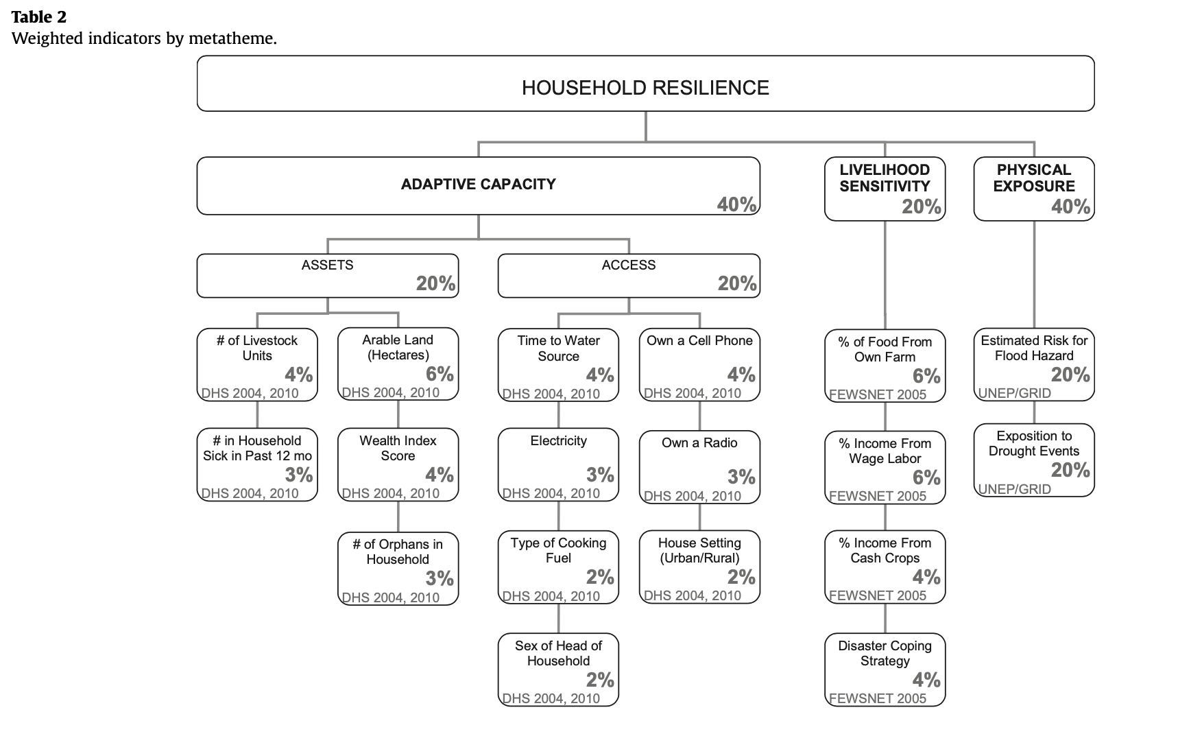Figure 1. Weighted indicators used to calculate adaptive capacity scores by metatheme, from Malcomb et al. (2014) (Table 2).

Finally, we georeferenced Figures 4 and 5 from Malcomb et al. (2014) in QGIS in order to compare the original study results to those produced by the above R script. This comparison was quantitatively demonstrated through a Spearman’s Rho correlation test.

Reproduction Results

The effort of this replication study appears to support the original findings of the Malcomb et al. (2014) paper we set out to validate. Our workflow produced the adaptive capacity scores seen in Figure 2, which strongly agree with those generated by Malcomb et al. (Figure 4). The difference map, illustrating the similarity between adaptive capacity scores for each Traditional Capacity scores, is seen in Figure 3, and highlights the similarities between the two maps and workflows. To support this similarity, this reproduction ran a Spearman’s Rho correlation test, resulting in the matrix seen in Table 3 and a rho value of 0.786.

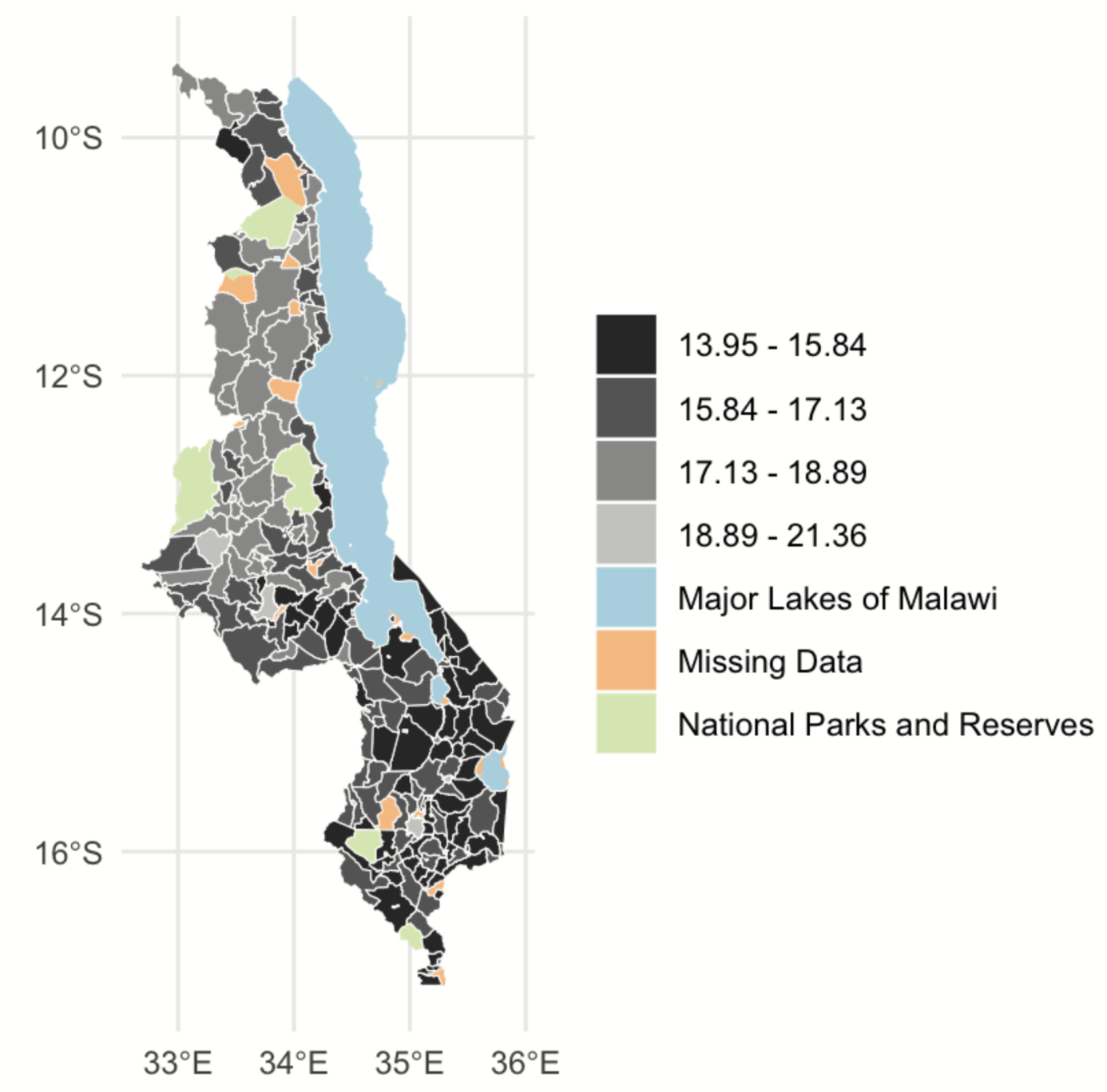Figure 2. Adaptive Capacity Scores from our reproduction results (mapping access and assets data). Data based on 2010 DHS surveys.

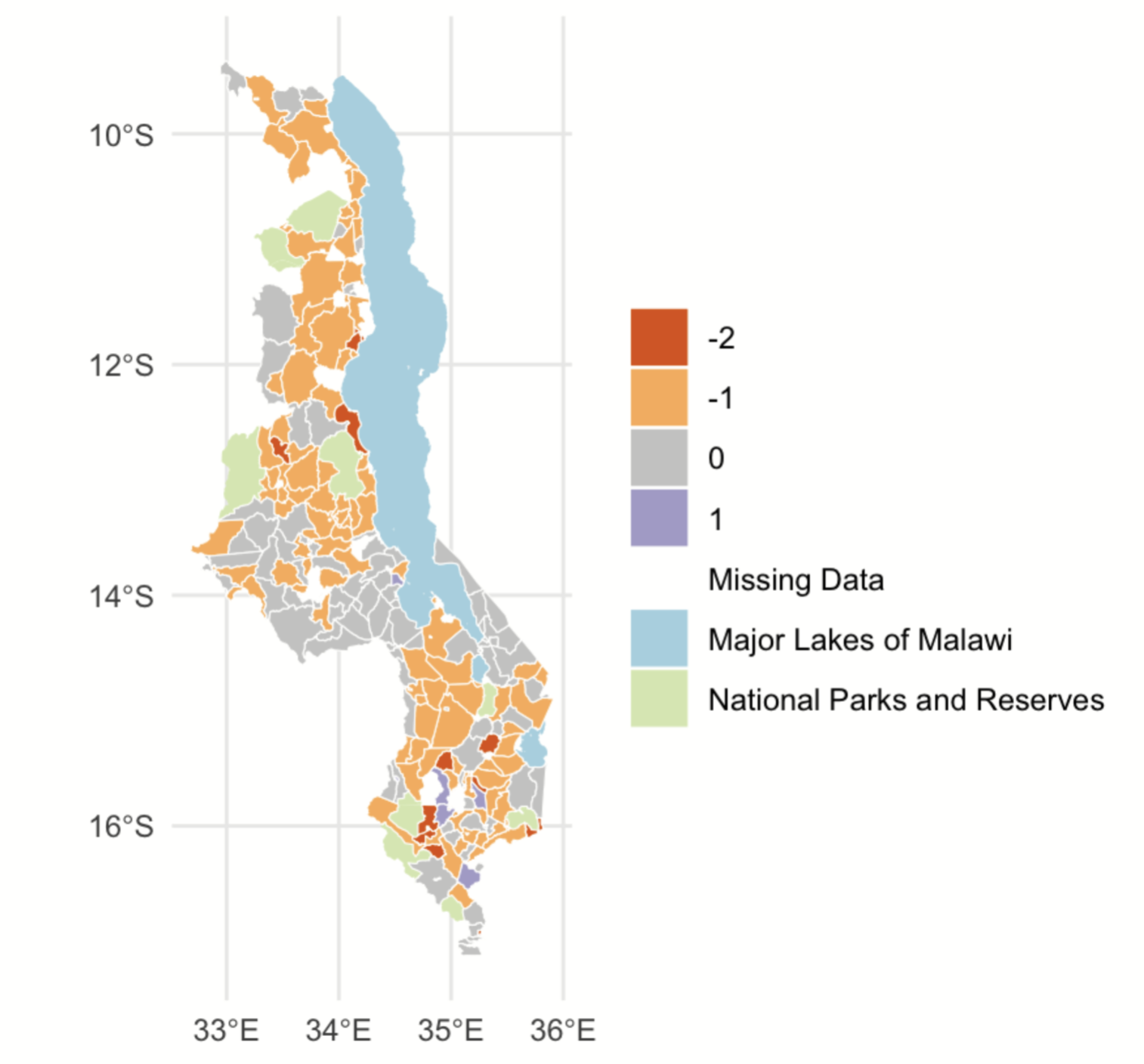Figure 3. Comparing Adaptive Capacity Score maps from our procedure (Fig 2) and from Malcomb et al. (2014) (Fig 4).

Table 3. Spearman’s rho correlation test results. (rho = 0.7856613). The results of the original study are shown on the x axis (columns), while the results of the reproduction are shown on the y axis (rows).

	1	2	3	4
1	34	5	0	0
2	25	25	0	0
3	5	43	20	0
4	0	7	27	5

When it came time to reproduce the vulnerability scores generated by Malcomb et al., however, our study was less successful. Our Vulnerability Scores map, seen in Figure 4 below, yielded a significant amount of disagreement with the figure produced by Malcomb et al. This comparison may be seen in Figure 5, where the high degree of red indicates a high degree of negative difference in vulnerability scores. A scatterplot comparing the scores from each study may be found in Figure 6, and another Spearman’s rho correlation test was performed to produce the low value of 0.202. In Figure 6, a linear relationship between points would have indicated a strong correlation between studies; however, as demonstrated, this correlation was not found.

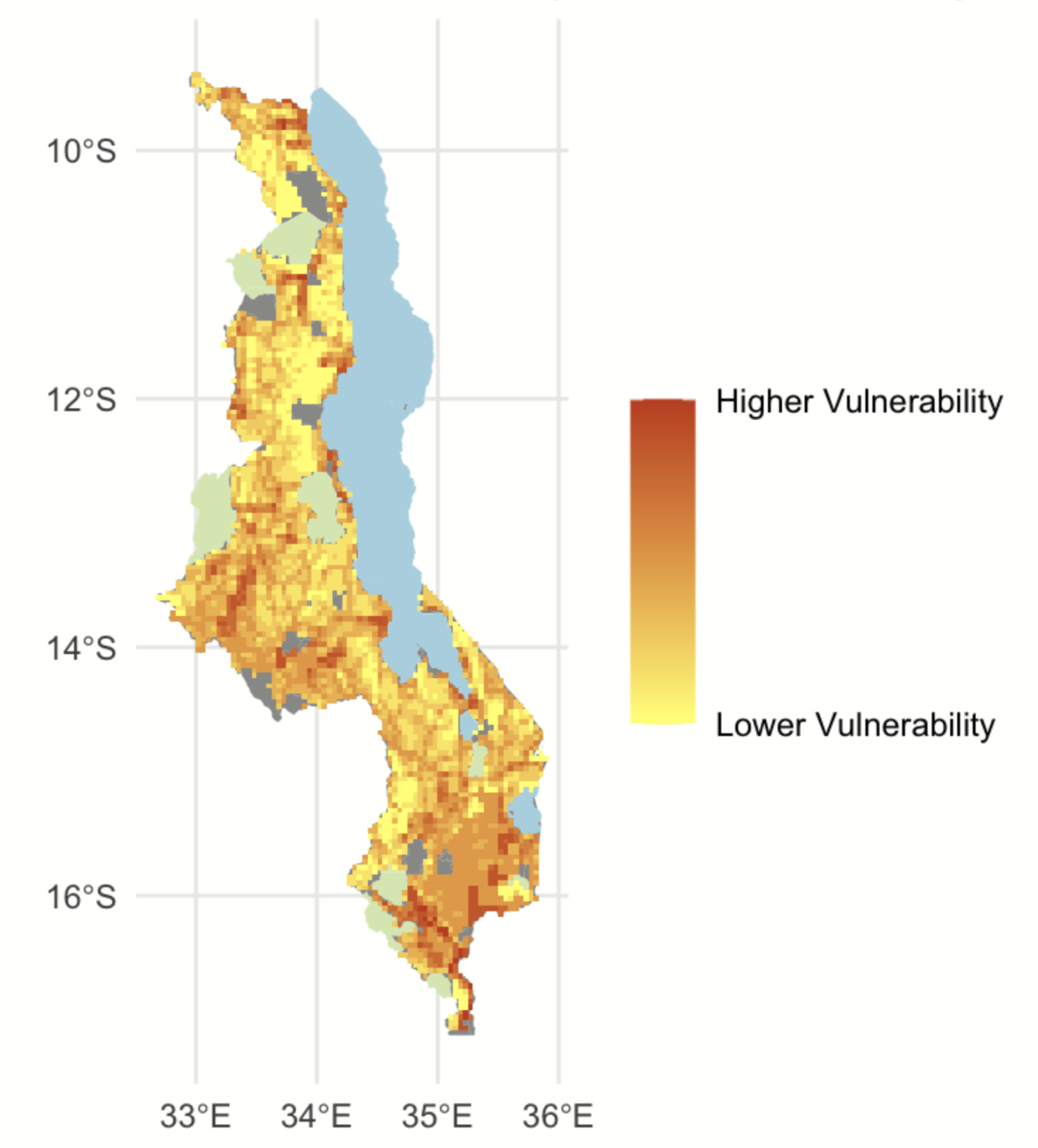Figure 4. Vulnerability Scores in Malawi from our reproduction results.

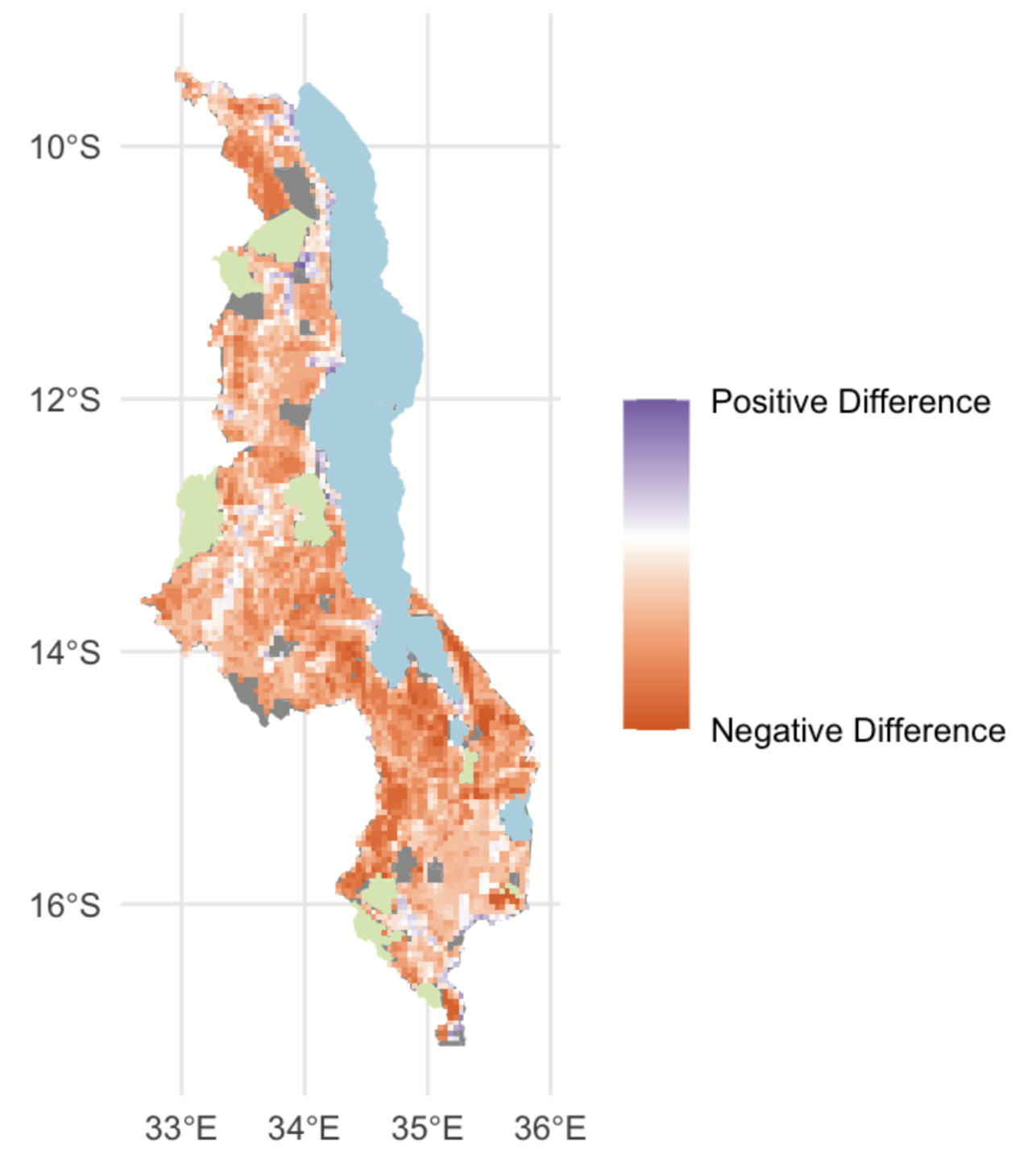Figure 5. Comparing Vulnerability Scores maps from our procedure (Fig 4) and Malcomb et al. (2014) (Fig 5).

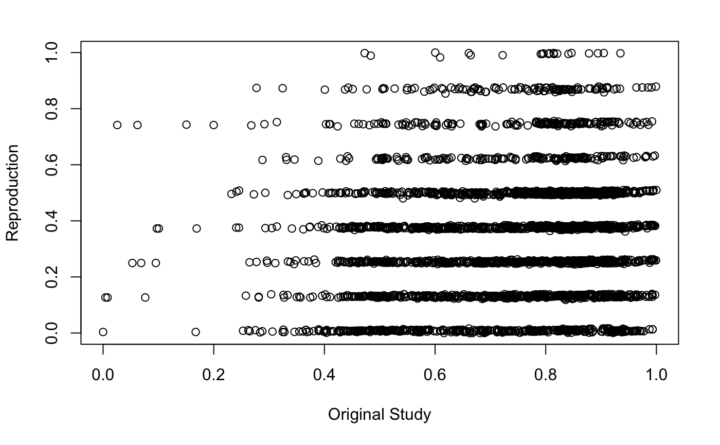Figure 6. A scatterplot comparing final vulnerability scores generated from the workflow of this reproduction and the results of the workflow of Malcomb et al. (2014). To achieve these scores, we used the formula difference = reproduction score - original score. A Spearman’s rho value resulted in 0.202.

Unplanned Deviations from the Protocol

This reproduction was structured so as to specifically highlight how our workflow changed as we gained more and more access to the datasources and workflow utilized in the original Malcomb et al. (2014) study. Therefore, our workflow saw many significant deviations from its initial state, with each major deviation being documented in the form of a new GitHub repository release.

The first challenges came as we first attempted to construct a workflow from the Malcomb et al. (2014), with no access to data. For example, our lab group was unsure of the scale of the DHS data to be used (village, household, district), as well as the specific methodologies for creating quintiles through which to score resiliency. The original study states it used categories 0 through 5 to represent quintiles, despite presenting 6 categories. In this reproduction, we favored quintiles and assigned categories 1 through 5. A similar issue again arose when deciding how to assign binary variables, such as sex of head of household, a rank along the 1-5 scale. Eventually, we opted to assign a value of 1 to males (the presumed lower-risk category) and 2 to females.

A final source of uncertainty came from the livelihood scores, which contained 4 indicators that were difficult to objectively quantify. Of these variables (see Table 2), “Disaster Coping Strategy” was particularly difficult to score, and little to no direction was provided by Malcomb et al. in their study. This data was incredibly rich and came in multiple scales and categories (for example, data came in poor, medium-income, rich sheets), and Malcomb et al. never specified from where or with what variables they calculated their livelihood scores. Our reproduction aims to improve on this direction with more specific methods seen in Table 2 above.

Discussion

This reproduction study succeeded in producing Malawi Traditional Authority Adaptive Capacity Scores similar to the original findings of Malcomb et al. (2014), but was unable to produce satisfactorily similar Vulnerability Scores.

As seen in Figures 2 and 3, Adaptive Capacity Scores for individual Traditional Authorities produced in this reproduction study share a strong correlation with those determined by Malcomb et al. in their results. It should be noted that one contributor to this similarity is the arbitrary multiplication of results by the constant 20, which increased the values of the scores into the range they are presented in in Figure 2 (around 14 to 22). I made the conscious decision to include this arbitrary constant in the final Adaptive Capacity Scores formula, even while some of my classmates did not. Neither camp is correct in their workflow, as the constant is purely to change the resulting integer displayed in the map.

It may have been because of this inclusion of the constant, however, that my comparison tests resulted in such similar products. The difference between Adaptive Capacity Scores per Traditional Authority may be seen in Figure 3, and it is evident there that many of these zones share the same score or are only different by +/- 1. This similarity is overall unsurprising, as we used the exact same dataset and clear variables from the DHS survey data as Malcomb et al. in their analysis. The Spearman’s rho correlation test serves as more evidence of this agreement, and the strong value of 0.786 indicates similar results.

We faced almost completely opposite reproduction conditions when attempting to recreate the Vulnerability Scores map. Malcomb et al. left almost their entire workflow up to broad interpretation, and we were left to determine for our own which variables to use, from which specific datasets, and in what part of the final indicator values used to calculate the final scores. Eventually, our group constructed our own categories with the specific variables seen in Table 2.

As a result of this new interpretation, our Vulnerability Score Map (Figure 4) did not share a very strong agreement with that produced by Malcomb et al. This comparison is illustrated in Figure 5, where the strong red presence indicates significant negative difference between maps. This lack of similarity is quantified through another Spearman’s rho test, which produced a result of 0.202. The lack of clarity in Malcomb et al.’s workflow was, while for the most part surmountable, ultimately the major hindrance in completing a full reproduction. Here, we have strived to fill in the gaps we found were missing from the original study, and we hope this information allows for the total reproduction of future sub-national climate analyses.

Conclusion

In conclusion, our reproduction effort working on recreating a sub-national climate vulnerability analysis first produced by Malcomb et al. in 2014 was only partially successful. This study was able to reproduce Adaptive Capacity Scores that strongly agree with those in the original study, yet was not able to reproduce anything significantly similar to the Vulnerability Scores figure. The most significant challenges were encountered when attempting to assign different variables within the available data to certain places in formulas utilized by Malcomb et al., as the original study did a good job outlining how the data was used, but not which aspects of the data were used.

We faced significant challenges in accurately reproducing the workflow to properly create the maps and figures we saw in Malcomb et al.’s publication, despite having access to 100% of the data and the entire paper. While some of these challenges were passable with time and increased collaboration, more were not and instead relied on our individual initiative to draw feasible workflows with the data available and only a rough idea of what an outcome should look like.

Our efforts cast a new light on the importance of clear and accessible methodologies, and the impact these sections of scientific publications can have on the validity of the science as a whole. Ensuring climate adaption model studies such as this will certainly hold paramount importance in the years to come, as climate change becomes an even more pressing issue and more and more countries around the world find the need to conduct thorough vulnerability assessments in the same manner as this study. If anything has been learned from this reproduction effort, it is that small details matter just as much as large ones, and clarifying datasets used is not helpful if specific variables that contribute to results are not highlighted. A final issue that is pertinent to this study (and will likely be for many future geospatial studies, as various code languages become more integrated into GIS analyses) is the benefits of including direct code in methodologies, in some form or another: this issue may still be a systemic hurdle, as the geospatial scientific community rewrites publication guidelines to accomodate new forms of analysis, but is a vital thought to hold and actively advocate in sharing future studies.

References

Malcomb, D. W., E. A. Weaver, and A. R. Krakowka. 2014. Vulnerability modeling for sub-Saharan Africa: An operationalized approach in Malawi. Applied Geography 48:17–30. DOI:10.1016/j.apgeog.2014.01.004

Report Template References & License

This template was developed by Peter Kedron and Joseph Holler with funding support from HEGS-2049837. This template is an adaptation of the ReScience Article Template Developed by N.P Rougier, released under a GPL version 3 license and available here: https://github.com/ReScience/template. Copyright © Nicolas Rougier and coauthors. It also draws inspiration from the pre-registration protocol of the Open Science Framework and the replication studies of Camerer et al. (2016, 2018). See https://osf.io/pfdyw/ and https://osf.io/bzm54/

Camerer, C. F., A. Dreber, E. Forsell, T.-H. Ho, J. Huber, M. Johannesson, M. Kirchler, J. Almenberg, A. Altmejd, T. Chan, E. Heikensten, F. Holzmeister, T. Imai, S. Isaksson, G. Nave, T. Pfeiffer, M. Razen, and H. Wu. 2016. Evaluating replicability of laboratory experiments in economics. Science 351 (6280):1433–1436. https://www.sciencemag.org/lookup/doi/10.1126/science.aaf0918.

Camerer, C. F., A. Dreber, F. Holzmeister, T.-H. Ho, J. Huber, M. Johannesson, M. Kirchler, G. Nave, B. A. Nosek, T. Pfeiffer, A. Altmejd, N. Buttrick, T. Chan, Y. Chen, E. Forsell, A. Gampa, E. Heikensten, L. Hummer, T. Imai, S. Isaksson, D. Manfredi, J. Rose, E.-J. Wagenmakers, and H. Wu. 2018. Evaluating the replicability of social science experiments in Nature and Science between 2010 and 2015. Nature Human Behaviour 2 (9):637–644. http://www.nature.com/articles/s41562-018-0399-z.

Main Page