Spatial Urban Climate Resilience Analysis in Dar es Salaam

Analysis and Application of Publicly-Collected Big Data in Sub-Saharan Africa

Produced by Nick Nonnenmacher

Created 03/31/2021 Revised 04/13/2021

Background Question

Understanding and improving urban resilience around the world is paramount in preparing human population hubs for changing climates in the near future. In this analysis, I implemented SQL queries in PostGIS to analyze and better understand certain aspects of urban resilience in the eastern African city of Dar es Salaam, Tanzania. I was interested in how urban green space affected population spatial distribution, so through using residential building spatial information as a proxy for population, my guiding question was, “is building density greater in areas closer to urban green space compared to farther away?”

Data

The data for this exercise was obtained from Open Street Map (OSM) and the Resilience Academy.

OSM is an open source public mapping effort aimed at creating accessible and accurate mapping data all over the world. Data is contributed by local parties and may be of any type. OSM data is tagged with a timestamp and username, and so it appears much of the data used in this analysis was contributed by members of Ramani Huria, a local Dar es Salaam mapping effort focused on collecting flood data and improving the city’s flood resilience.

Ramani Huria itself is just one initiative of the larger organization the Resilience Academy, a program bringing together five academic institutions in Tanzania and Finland in order to improve social capacity to tackle changing climate and urban challenges. Resilience Academy is providing inclusive and comprehensive mapping and digital knowledge, skills, and tools to students and partners, with the aim of improving urban planning and design, climate response models and practices, and infrastructure for developing cities in Tanzania and beyond.

Specific data used in this analysis includes:

• wards: adminstrative wards in Dar es Salaam, 2018
• landuse: land use in Dar es Salaam, 2019
• buildings: buildings in Dar es Salaam, 2019

Methods

This exercise was as much an exercise in SQL literacy and open-source science as an analysis in urban resilience. Therefore, extra effort has been allocated into developing an accessible and reproducible workflow that can be replicated in PostGIS - using the OSM2PGSQL tool - and used as an effective SQL teaching mechanism.

The first step to this analysis was obtaining data from the Resilience Academy and OSM. Joe Holler, the professor of this class, had already obtained and downloaded Dar es Salaam ward and building data, which I accessed in PostGIS using the DB Manager tool in QGIS.

Next, I created new tables in my personal schema containing building and greenspace information. Since the only population data available at a reasonable scale was very dated, I used residential buildings as a proxy for population. To filter these buildings, I created a new table called darbuildings from the building field of the plant_osm_polygon layer taken from OSM, which contained over 1.3 million features. Isolating greenspace was a bit more difficult, because various attributes that could have been considered greenspace were scattered throughout multiple different fields in plant_osm_polygon. I ended up selecting specific attributes ‘greenfield’, ‘park’, ‘grass’, ‘recreation ground’, ‘garden’, ‘wood’, ‘tree’, ‘beach’, ‘tree_row’, and ‘grassland’ from three different fields: ‘landuse’, ‘leisure’, and ‘natural’. Once I had isolated these attributes within their individual fields, I was able to combine the three subsequent tables into one ‘greenspace’ table containing points of each attribute. This table contained 356 rows.

Create new tables in personal schema

CREATE TABLE darbuildings AS
SELECT osm_id, st_transform(way,32737)::geometry(polygon,32737) as geom, name
FROM planet_osm_polygon
WHERE building ILIKE 'residential' OR 'yes';

/* this first table contains all the building attributes labeled "residential" or "YES" */

CREATE TABLE landusespace2 AS
SELECT osm_id, landuse, st_transform(way,32737)::geometry(polygon,32737) as geom, name
FROM planet_osm_polygon
WHERE landuse = 'greenfield' OR landuse = 'park' OR landuse = 'grass' OR landuse = 'recreation ground';

CREATE TABLE leisurespace AS
SELECT osm_id, leisure, st_transform(way,32737)::geometry(polygon,32737) as geom, name
FROM planet_osm_polygon
WHERE leisure = 'garden' OR leisure = 'park';

CREATE TABLE naturalspace AS
SELECT osm_id, "natural", st_transform(way,32737)::geometry(polygon,32737) as geom, name
FROM planet_osm_polygon
WHERE "natural" = 'wood' OR "natural" = 'tree' OR "natural" = 'beach' OR "natural" = 'tree_row' OR "natural" = 'grassland' OR "natural" = 'grass';

I used this query to search within the three fields that would contribute to the ‘greenspace’ table (‘landuse’, ‘leisure’, and ‘natural’). The term field1 represents the specific field I was searching in. This query helped me determine which attributes I should include in the three pull queries above. Unfortunately, I had to leave many attributes out of this analysis, and did not have an objective selection technique. Nearly 60 such attributes were therefore not included as greenspace in Dar es Salaam, and included such features as reefs, cemeteries, reservoirs, and farmland.

SELECT field1, count(osm_id) as n
FROM planet_osm_polygon
GROUP BY field1
ORDER BY n DESC;

Once the residential buildings and appropriate greenspace features had been isolated, I created the buffer zones around each greenspace point in the city. I chose the arbitrary distance of 500m to create these buffers. By dissolving overlapping buffers, I would later be able to calculate area and building density. This process resulted in 42 buffer features, from the 356 unique greenspace points.

CREATE TABLE greenspacecentroids AS
SELECT osm_id, st_centroid(geom)::geometry(point,32737) as geom from greenspace;

/* create centroids in each polygon attribute */

CREATE TABLE greenspacebuffer AS
SELECT osm_id, st_buffer(geom, 500)::geometry(polygon,32737) as geom from greenspacecentroids
UNION
SELECT osm_id, st_buffer(geom, 500)::geometry(polygon,32737) as geom from greenspace;

/* create buffers */

CREATE TABLE greenspacebufferdissolve AS
SELECT st_union(geom)::geometry(multipolygon,32737) AS geom
FROM greenspacebuffer;

/* dissolve into one layer */

CREATE TABLE greenspacebuffers AS
SELECT (st_dump(geom)).geom::geometry(polygon,32737)
FROM greenspacebufferdissolve;

/* multipart to single parts */

/* greenspacebuffers = 42 features */

ALTER TABLE greenspacebuffers ADD COLUMN id SERIAL PRIMARY KEY;

/* give each buffer a unique id based off column number */

Next, I distinguished which buildings were inside and outside the buffer zones. It is immediately evident that many more buildings sit outside the buffer zones than inside.

ALTER TABLE darbuildings
ADD COLUMN greenbuffer

UPDATE darbuildings
SET greenbuffer = 1
FROM greenspacebuffers
WHERE st_intersects(darbuildings.geom, greenspacebuffers.geom);

SELECT greenbuffer, count(osm_id) as n
FROM darbuildings
GROUP BY greenbuffer
ORDER BY n DESC;

/*
now we explicitly know which buildings are within the buffer zones and which aren't
total features in darbuilings = 1,358,546
features within buffer zones = 266,142
features outside buffer zones = 1,092,527
*/

Then, I calculated the total city area inside each of the 42 buffer zones, and the total city area of each of the 95 individual city wards. Both areas are represented in 1000m2.

ALTER TABLE greenspacebuffers
ADD COLUMN area_km2_buffers real;

UPDATE greenspacebuffers
SET area_km2_buffers = st_area(geom) / 1000;

/* this will give us the area of each of the 42 buffer zones in square kilometers*/

ALTER TABLE wards2
ADD COLUMN area_km2 real;

UPDATE wards2
SET area_km2 = st_area(utmgeom)/1000;

/* this will give us the area of each of the 95 city wards  */

The next step was the join the building points and buffer polygons. This was done with an intersect.

CREATE TABLE pop_density_green AS
SELECT
greenspacebuffers.id as id, greenspacebuffers.geom as geom1,
COUNT(darbuildings.greenbuffer) as total_ct
FROM greenspacebuffers
JOIN darbuildings
ON st_intersects(darbuildings.geom, greenspacebuffers.geom)
GROUP BY greenspacebuffers.id;

Now, I know the area in 1000 square meters and the number of buildings within the 42 buffer zones, contained in the ‘pop_density_green’ table, and the area in 1000 square meters and the number of buildings within the 95 city wards, contained in the ‘wards2’ table. It only takes a simple calculation from here to create a new building density column!

ALTER TABLE pop_density_green
ADD COLUMN density_inside real;

UPDATE pop_density_green
SET density_inside = pop_density_green.total_ct / pop_density_green.area_km2_inside;

ALTER TABLE wards2
ADD COLUMN percent_flooded real;

UPDATE ward_flood2
SET pop_density = wards2.totalpop / wards2.area_km2;

The final step, in order to visualize all of my results in the spatial frame of the census wards, was to determine the ratio of buildings close to urban greenspace (ie, buildings within the 500m buffer zone) to buildings far from urban greenspace, by each ward. This was done through another join function, similar to when I joined building points and buffer zones, followed by a simple ratio calculation.

CREATE TABLE ward_ratio2 AS
SELECT
wards2.id as id, wards2.utmgeom as geom1,
COUNT(darbuildings.greenbuffer) as near_green_buildings,
COUNT(darbuildings.osm_id) as far_green_buildings
FROM wards2
JOIN darbuildings
ON st_intersects(darbuildings.geom, wards2.utmgeom)
GROUP BY wards2.id;

ALTER TABLE ward_ratio2
ADD COLUMN ratio real;

UPDATE ward_ratio2
SET ratio = ward_ratio2.near_green_buildings * 1.0  / ward_ratio2.far_green_buildings;

/* the field near_green_buildings was multiplied by 1.0 here in order for SQL to recognize the query as real number division */

From here, I added the ‘wards2’, ‘pop_density_green’, and ‘ward_ratio2’ layers into a QGIS file and created chloropleth maps from the building density data (Figures 1, 3, and 4). I also added the greenspace centroid points before buffers were added, to visualize where the urban green space actually is in the city in a separate map (Figure 2). An OSM Standard basemap was added to all four figures for easier viewing. Additionally, a Leaflet interactive map was created to better understand how building density changes in relation to ward and the presence of urban green spaces.

The .sql document containing all of my queries may be found here. The initial SQL exercise studying Dar es Salaam flood risk conducted by Joe Holler and the Middlebury College spring 2021 GEOG 323 class may be found here.

Results

Here is a map summarizing building density distribution in relation to green space in Dar es Salaam.

These results show that there is a general positive correlation between high-density wards and high-density buffer zones - implying urban green space does not significantly influence proximate building density. As seen in Figures 2 and 3, the highest-density wards are situated in the center of the city along the coastline, and overlap with the major cluster of urban green points. This is further supported in Figure 2, where the darkest-blue buffer zones are most represented in the same city center region.

Figure 4 displays the ratio of buildings in each ward close to versus farther away from urban greenspace areas. As evident by the darker green in the center of the city, higher percents of buildings are closer to urban green space where building density is higher, as well as where urban greenspace itself seems to be clustered. This visualization helps to contextualize the results of this analysis within the spatial framework of census wards, and shines a light on which wards have a higher access to greenspace and how that changes across the space of Dar es Salaam.

There are a few notable exceptions to this pattern. A range of third-quintile buffer zones are found just to the northeast of the city center clusters, representing a noticeable beachfront community. More examples may be seen in the western-most wards of the city, where a few fourth- and third-quintile buffer zones linger even as the overall ward density drops to second- and first-quintiles.

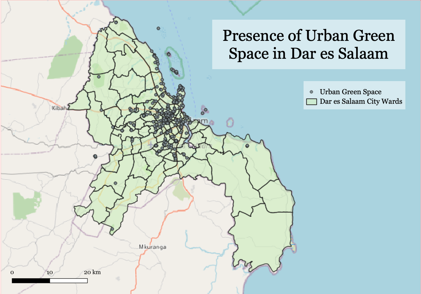Figure 1. Green space in Dar es Salaam in 2019, represented as points. Data obtained from Resilience Academy and OSM (Basemap: OSM).

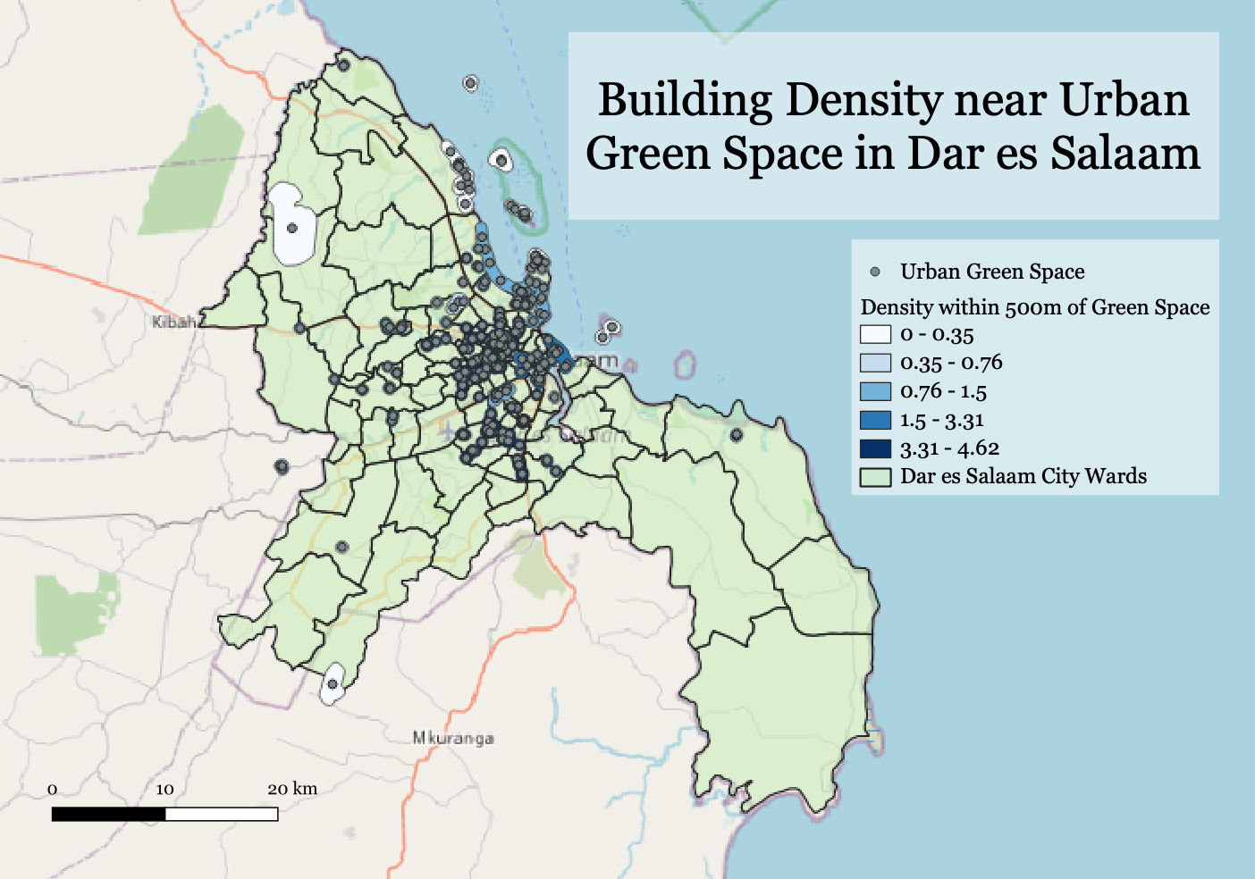Figure 2. Building density by green space buffer zone in Dar es Salaam in 2019. Data obtained from Resilience Academy and OSM (Basemap: OSM).

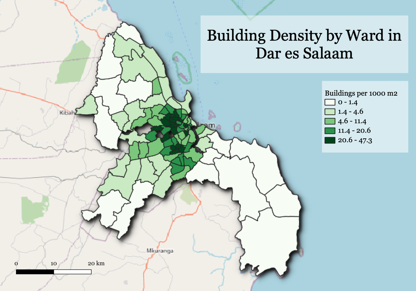Figure 3. Building density by city ward in Dar es Salaam in 2018. Data obtained from Resilience Academy and OSM (Basemap: OSM).

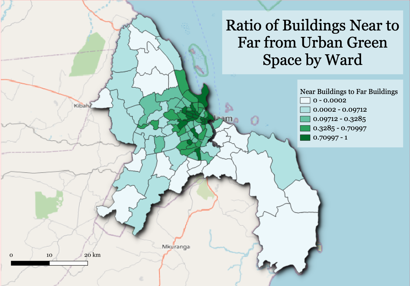Figure 4. The ratio of buildings near urban greenspace to buildings far from urban greenspace, delineated by ward. Data obtained from Resilience Academy and OSM (Basemap: OSM).

In conclusion, the results of this analysis simply suggest that urban green space has been incorporated in regions of the city where building density is already high. In addition, it is evident that urban greenspace has been concentrated among population density hotspots, near the center of the city. Past studies have demonstrated there may be direct and indirect human health benefits to increasing the abundance of nature and natural places in modern urban space (van Leeuwen, Nijkamp, and de Norohna Vaz 2011, Lee and Maheswaran 2011, De Ridder et al 2004), and this may prove even more significant in rapidly-developing cities such as Dar es Salaam. Green spaces have been shown to provide cooling effects in dense urban centers, enhance local air quality, and even improve the use of nearby farmland (van Leeuwen, Nijkamp, and de Norohna Vaz 2011). As Dar es Salaam continues to grow in size and population over the next decade, pointed effort must be devoted to the city’s infrastructure and use of natural resources in order to provide a safe and healthy economic and cultural hub for Tanzania and east Africa.

Acknowledgements

Thank you to Professor Joe Holler of Middlebury College for organizing this exercise and providing easily-accessible data and SQL exercises to aid myself and my GEOG 323 classmates in completing our analyses. Thank you also to my classmates for their help during this analysis. In addition, map data featured in this analysis is provided by OSM and the many users who contribute to it.

References

De Ridder, K., Adamec, V., Bañuleos, A., Bruse, M., Bürger, M., Damsgaard, O., Dufek, J., Hirsch, J., Lefebre, F., Pérez-Larcorzana, J.M., Thierry, A., and C. Weber. 2004. An integreated methodology to assess the benefits of urban green space. Science of the Total Environment 334-335:489-497. https://doi.org/10.1016/j.scitotenv.2004.04.054

Lee, A.C.K. and R. Maheswaran. 2011. The health benefits of urban green spaces: a review of the evidence. Journal of Public Health 33(5):212-222. https://doi.org/10.1093/pubmed/fdq068

Schuurman, N. 2008. Database Ethnographies Using Social Science Methodologies to Enhance Data Analysis and Interpretation. Geography Compass 2 (5):1529–1548. https://onlinelibrary.wiley.com/doi/abs/10.1111/j.1749-8198.2008.00150.x

van Leeuwen, E., Nijkamp, P., and T. de Norohna Vaz. 2011. The multifunctional use of urban green space. International Journal of Agricultural Sustainability 8(1-2):20-25. https://doi.org/10.3763/ijas.2009.0466

Main Page